Hey there, I’m Adam Drees and I’m located in Portland, OR. I manage and lead a software team which develops the embedded software used to run Hyster and Yale branded forklifts.
Previously, I worked as a Scrum Master and Embedded Software Engineer at Emerson in Charlottesville, VA where I developed embedded software for industrial controllers.
For several years, I worked as a Simulation Project Engineer with Emerson in Saint Louis, MO. I worked in the field of process simulation and control. My focus was building low-cost process simulations used for agricultural processing plants, pulp and paper, water/wastewater treatment and power generation. I also worked as an instructor who taught control engineers how to develop and maintain simulations.
In 2013, I earned a B.S in Mechanical Engineering at Missouri University of Science and Technology. From 2014 to 2018, I attended Computer Science courses at University of Missouri-Saint Louis. In 2021, I graduated from Georgia Institute of Technology with a M.S. in Computer Science.
My hobbies include rock climbing, mountain biking, hiking, and skiing.
In this video, I present on the paper Leave Your Phone at the Door: Side Channels that Reveal Factory Floor Secrets. This presentation is part is for the Cyber-Physical Systems Security class I am attending at Georgia Tech. The paper can be found at this link.
Natural Convection Simulation: Mathematical Model
Working on my undergraduate degree in Mechanical Engineering, my favorite class was heat transfer. For a class project, I built a simple simulation that showed convection for a randomly generated temperature field. At the time, I didn’t have enough programming skills to build a quality simulation. The purpose of this is to revisit that project with my improved science and programming skills. Along the way, I will teach the math behind building the model. The first step will be to research the fundamental equations for this system.
Problem Definition
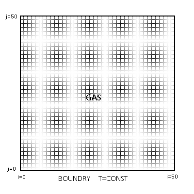
In this project, we will model a compressible fluid. Natural convection forces will affect the fluid. The simulation will model the transient behavior of a starting temperature or input heat. The simulation will be 2-Dimensional to display the results easier. Lastly, the model will use constant Cartesian cell structure to simplify the problem.
A conservation of energy equation was developed by including conduction, convection and external heat to the first law of thermodynamics
The ideal gas law will be used to determine pressure
Finite Difference Approximation
A finite difference approximation will be used to solve the fluid state at future time intervals. A small time step and cell size will be desired to maximize accuracy. Central difference approximations will be used to reduce any directional biases.
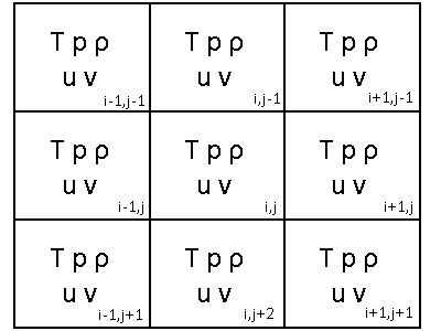
When using a finite difference, we can encounter a problem. The grid below uses the same cells to represent both pressure and velocity.
Since we are using a central difference approximation, the velocities of center square is based on the pressure difference between it’s neighbors. We can see how the equation does not compare the squares current pressure between it’s neighbor squares.
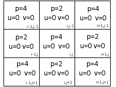
If there is not a pressure differential between the 2 opposite neighbor cells then we do not get flow. As a result, a checkerboard pattern will emerge. The image below shows a possible solution.
This solution solves the governing equations but creates a system that is unrealistic. In a real system, we would see flow from the 4-pressure elements into the 2-pressure elements.
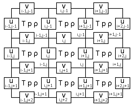
A better solution uses different, overlapping areas for the pressures and velocities. In the improved solution, the pressures exist in each area of the grid and the velocities represent the flows between the pressure cells. This solution is represented below.
Solved Equations
With our improved grid model, we can finally solve the governing equations using a finite difference approximation. The following equations can calculate the next simulation conditions based on the current conditions.
Navier-Stokes equations for velocity
Conservation of mass for density
Conservation of energy for temperature
Ideal gas law for pressure
These equations can directly be used in our simulation. Beyond these equations, we will have to consider the boundary conditions. The boundaries can be modeled in many different ways so we will review them later. With all that in mind, we can begin the design and development of our simulation.


 =-\frac { dp }{ dx } +\mu \left( \frac { { d }^{ 2 }u }{ { dx }^{ 2 } } +\frac { { d }^{ 2 }u }{ { dy }^{ 2 } } \right) +\rho { g }_{ x } \\ \rho \left( \frac { dv }{ dt } +u\frac { dv }{ dx } +v\frac { dv }{ dy } \right) =-\frac { dp }{ dy } +\mu \left( \frac { { d }^{ 2 }v }{ { dx }^{ 2 } } +\frac { { d }^{ 2 }v }{ { dy }^{ 2 } } \right) +\rho { g }_{ y }")
 =0")
 =k\left( \frac { { d }^{ 2 }T }{ { dx }^{ 2 } } +\frac { { d }^{ 2 }T }{ { dy }^{ 2 } } \right) +S")

 +{ g }_{ x }-{ u }_{ i,j }^{ t }\frac { { u }_{ i+1,j }^{ t }-{ u }_{ i-1,j }^{ t } }{ 2\Delta x } -{ v }_{ i,j }^{ t }\frac { { u }_{ i,j+1 }^{ t }-{ u }_{ i,j-1 }^{ t } }{ 2\Delta y } \right)")
 +{ g }_{ x }-{ u }_{ i,j }^{ t }\frac { { u }_{ i+1,j }^{ t }-{ u }_{ i-1,j }^{ t } }{ 2\Delta x } -\left( { v }_{ i,j }^{ t }+{ v }_{ i-1,j }^{ t } \right) \frac { \left( { u }_{ i,j }^{ t }-{ u }_{ i,j-1 }^{ t } \right) }{ 4\Delta y } -\left( { v }_{ i,j+1 }^{ t }+{ v }_{ i-1,j+1 }^{ t } \right) \frac { \left( { u }_{ i,j+1 }^{ t }-{ u }_{ i,j }^{ t } \right) }{ 4\Delta y } \right) \\ { v }_{ i,j }^{ t+1 }=v_{ i,j }^{ t }+\Delta t\left( -\frac { { p }_{ i,j }^{ t }-{ p }_{ i,j-1 }^{ t } }{ \rho \Delta y } +\frac { \mu }{ \rho } \left( \frac { { v }_{ i+1,j }^{ t }+{ v }_{ i-1,j }^{ t }-2v_{ i,j }^{ t } }{ { \Delta x }^{ 2 } } +\frac { { v }_{ i,j+1 }^{ t }+{ v }_{ i,j-1 }^{ t }-2v_{ i,j }^{ t } }{ { \Delta y }^{ 2 } } \right) +{ g }_{ y }-{ v }_{ i,j }^{ t }\frac { { v }_{ i,j+1 }^{ t }-{ v }_{ i,j-1 }^{ t } }{ 2\Delta y } -\left( { u }_{ i,j }^{ t }+{ u }_{ i,j-1 }^{ t } \right) \frac { \left( { v }_{ i,j }^{ t }-{ v }_{ i-1,j }^{ t } \right) }{ 4\Delta x } -\left( { u }_{ i+1,j }^{ t }+{ u }_{ i+1,j-1 }^{ t } \right) \frac { \left( { v }_{ i+1,j }^{ t }-{ v }_{ i,j }^{ t } \right) }{ 4\Delta x } \right)")
 +\frac { u_{ i+1,j }^{ t } }{ \Delta x } \left( \rho _{ i,j }^{ t }+\rho _{ i,j-1 }^{ t } \right) +\frac { v_{ i,j }^{ t } }{ \Delta y } \left( \rho _{ i,j }^{ t }+\rho _{ i+1,j }^{ t } \right) -\frac { v_{ i,j+1 }^{ t } }{ \Delta y } \left( \rho _{ i,j }^{ t }+\rho _{ i,j+1 }^{ t } \right) \right)")
 \left( \rho _{ i-1,j }^{ t }+\rho _{ i,j }^{ t } \right) +\frac { u_{ i+1,j }^{ t } }{ 2\Delta x } \left( T_{ i+1,j }^{ t }-T_{ i,j }^{ t } \right) \left( \rho _{ i+1,j }^{ t }+\rho _{ i,j }^{ t } \right) +\frac { v_{ i,j }^{ t } }{ 2\Delta y } \left( T_{ i,j-1 }^{ t }-T_{ i,j }^{ t } \right) \left( \rho _{ i,j-1 }^{ t }+\rho _{ i,j }^{ t } \right) +\frac { v_{ i,j+1 }^{ t } }{ 2\Delta y } \left( T_{ i,j+1 }^{ t }-T_{ i,j }^{ t } \right) \left( \rho _{ i,j+1 }^{ t }+\rho _{ i,j }^{ t } \right) +\frac { k }{ { C }_{ v } } \left( \frac { T_{ i-1,j }^{ t }+T_{ i+1,j }^{ t }-2T_{ i,j }^{ t } }{ { \Delta x }^{ 2 } } +\frac { T_{ i,j-1 }^{ t }+T_{ i,j+1 }^{ t }-2T_{ i,j }^{ t } }{ { \Delta y }^{ 2 } } \right) +{ S }_{ i,j } \right)")

 \\ \rho =Density\quad \left( \frac { kg }{ { m }^{ 3 } } \right) \\ p=Pressure\quad \left( Pa \right) \\ \mu =Dynamic\quad Viscosity\quad \left( \frac { kg }{ m\cdot s } \right) \\ T=Temperature\quad \left( K \right) \\ g=Gravitational\quad Acceleration\quad \left( \frac { m }{ { s }^{ 2 } } \right) \\ { R }_{ specific }=Ideal\quad Gas\quad Constant\quad \left( \frac { J }{ kg\cdot K } \right) \\ { C }_{ v }=Heat\quad Capacity\quad at\quad Constant\quad Volume\quad \left( \frac { J }{ kg\cdot K } \right) \\ S=External\quad Heat\quad \left( \frac { J }{ { m }^{ 3 }s } \right)")